Economic Order Quantity: Finding Your Optimal Order Size

Are you tired of guessing how much inventory to buy? Finding your economic order quantity is the specific answer you have been looking for. While basic summaries might mention it as a simple concept, we are going to look at the exact mechanics that allow you to minimize costs and maximize efficiency. This is the detailed breakdown you have been searching for to stop wasting money on warehouse space or excessive shipping fees. Ready for the specifics?

When it comes to managing stock, most businesses struggle with a constant tug-of-war. If you buy too much, your cash is locked up in boxes sitting on a shelf. If you buy too little, you are constantly paying for new shipments and risking stockouts. The EOQ model exists to settle this conflict. We are going to get straight into what works, what does not, and exactly what you should do to find your optimal order quantity. For a complete overview of the broader landscape of stock control, check out our main guide on the best inventory management methods. Let us get into the details.

The Core Logic of Economic Order Quantity

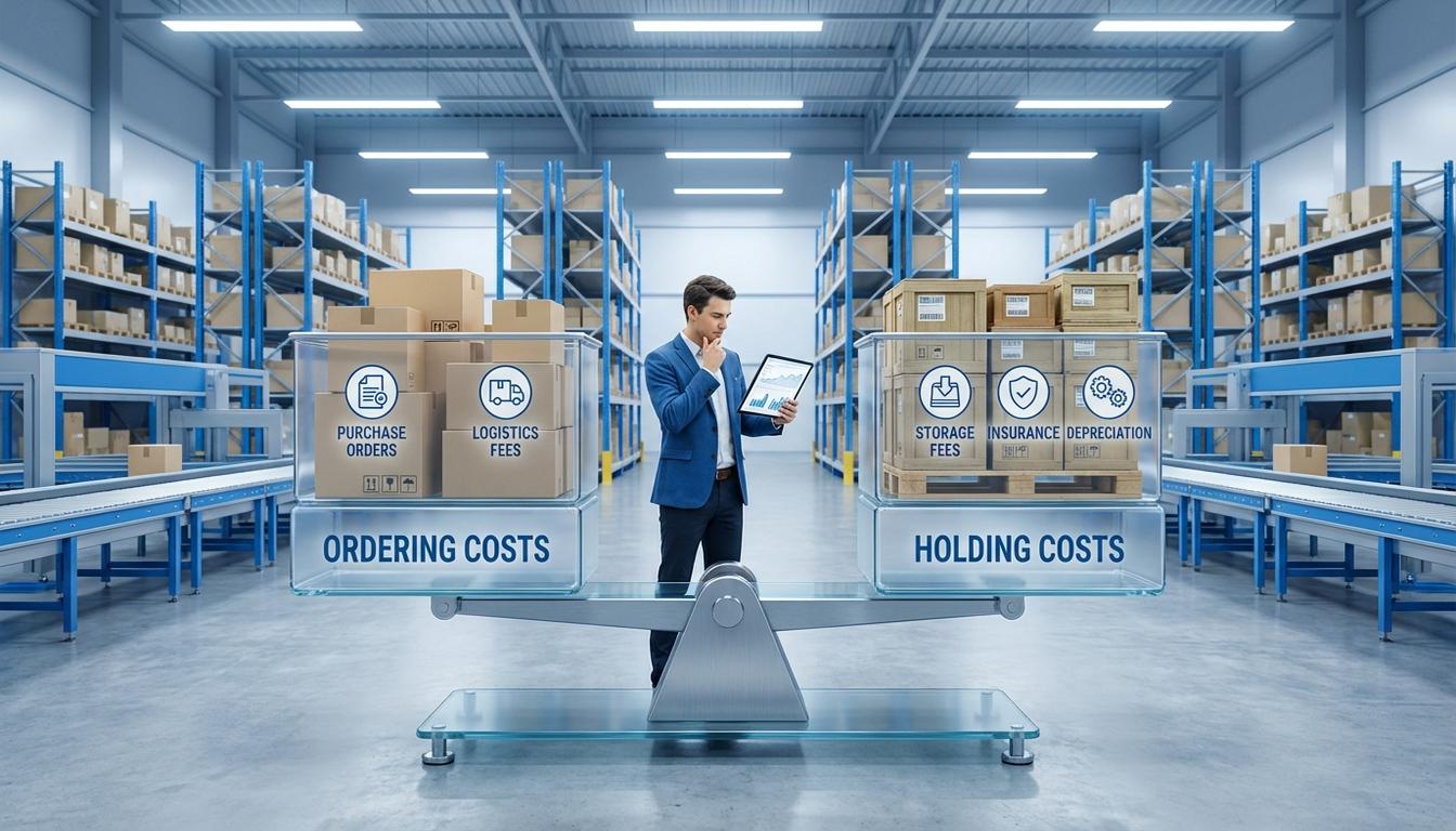
The economic order quantity is not just a math formula. It is a strategic balance point. We use it to find the exact order size that minimizes the total annual cost of ordering and holding inventory. This concept is also known as the economic lot size or the Wilson EOQ formula. The logic is built on a specific trade-off between two main cost categories that naturally move in opposite directions.

First, we have ordering costs. These are the fixed costs you pay every time you place and receive an order. Think about the administrative time spent creating a purchase order, the shipping fees, the handling costs at the loading dock, and the time spent inspecting the goods. If you place many small orders throughout the year, these costs skyrocket. Here is the specific situation where this applies. A company ordering 10 units every week pays for shipping 52 times. That is a lot of overhead.

Second, we have holding costs. These are also called carrying costs. This is what it costs you to keep one unit in stock for a full year. It includes warehouse rent, utilities, insurance, and the capital cost of the money tied up in that inventory. It also accounts for depreciation and the risk that the item might become obsolete or damaged while sitting around. When you place one massive order to save on shipping, your average inventory levels go up. This means your holding costs also go up. The optimal order quantity is the point where these two costs are perfectly balanced. The practical takeaway is that at this specific point, your total annual inventory cost is at its absolute minimum.

Breaking Down the EOQ Formula

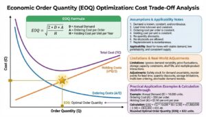
To use this tool effectively, we need to understand the variables involved. We are looking for the order quantity that makes the annual ordering cost equal to the annual holding cost. When these two numbers meet, the total cost curve is at its lowest point. Let us look at this closely. The standard EOQ formula is expressed as follows.

EOQ = √((2 * D * S) / H)

Here is what those letters actually represent in your day-to-day operations.

• D (Annual Demand): This is the total number of units you expect to sell or use over a one-year period. You should base this on historical sales data or confirmed forecasts. Accuracy here is vital.
• S (Ordering Cost): This is the fixed cost per purchase order. It does not matter if you order 5 units or 500 units. The cost to process the paperwork and pay the base shipping fee remains the same.
• H (Holding Cost): This is the annual cost of holding one unit in inventory. Often, businesses calculate this as a percentage of the item’s purchase price. For example, if an item costs $100 and your annual carrying rate is 20%, your H would be $20.

The EOQ calculation works by multiplying the demand and ordering cost by two, then dividing that by the holding cost. Finally, we take the square root of the whole thing. The square root is what allows the formula to find that specific “sweet spot” on the curve where costs are minimized. According to the Corporate Finance Institute, this formula is a foundational element of inventory optimization that helps businesses maintain healthy cash flow.

A Practical Example of EOQ in Action

Let us get specific here. Imagine a business that sells specialized industrial filters. Here is the data for one of their top-selling items.

• Annual Demand (D): 10,000 filters
• Ordering Cost (S): $500 per order
• Holding Cost (H): $0.75 per filter, per year

Using our EOQ model, we perform the following steps. First, we multiply 2 by 10,000, then by 500. This gives us 10,000,000. Next, we divide 10,000,000 by 0.75, which results in approximately 13,333,333. Finally, we take the square root of that number. The result is approximately 3,652 units.

What does this mean for you? If you order 3,652 filters at a time, you will minimize your total costs. If you order more than that, your warehouse costs will climb faster than your shipping savings. If you order less, the repetitive shipping and processing fees will outweigh the savings in storage. In this case, the company would place roughly three orders per year to meet its 10,000-unit demand. This level of order quantity optimization ensures you aren’t leaving money on the table. It is one of those areas where getting it right makes a real difference in your annual profit margins.

Key Assumptions of the Classic EOQ Model

There is a reason this specific aspect confuses people. They try to apply the basic formula to a messy, unpredictable world and wonder why the results feel off. The classic economic order quantity model relies on several simplifying assumptions. You need to know these so you can adjust your strategy when reality interferes.

One major assumption is that demand is constant and known. In the model, the business sells the exact same number of units every single day. There are no seasonal spikes and no random surges. Another assumption is that lead time is constant. This means that from the moment you click “order,” it takes the exact same number of days for the goods to arrive every single time. The model also assumes instantaneous replenishment. The moment the shipment arrives, your inventory level jumps from zero to your full optimal order quantity.

Furthermore, the model assumes you never run out of stock and that the unit price is constant. It does not account for quantity discounts or price fluctuations. While these assumptions sound restrictive, they make the EOQ a powerful baseline. Once you have this baseline, you can layer on more complex strategies. For instance, you might combine your order quantity with a safety stock calculation to handle the reality of variable demand. This is exactly what you need to know to move from theoretical math to practical application.

Advanced Variants and Quantity Discounts

The short version is that the basic formula is a starting point, but most suppliers offer price breaks. If your supplier says, “We will give you 10% off if you order 5,000 units,” the standard EOQ calculation might tell you to only order 3,652. This is where the detail changes everything. To handle quantity discounts, you have to compare the total annual cost of the EOQ quantity against the total annual cost of the discount threshold.

When calculating total cost with discounts, you must include the actual purchase price of the items. In the basic EOQ model, we often ignore the purchase price because it stays the same regardless of order size. But with discounts, the unit price (C) becomes a variable. You would calculate the total cost for each price bracket using the formula: Total Cost = (Ordering Cost) + (Holding Cost) + (Purchase Cost). Your best move here is to choose the quantity that results in the lowest overall number, even if it is higher than the initial EOQ result.

Another common variant is the Economic Production Quantity (EPQ). This applies when you are manufacturing the items yourself rather than buying them from a supplier. Instead of the inventory arriving all at once, it builds up gradually as it is produced. The EPQ formula adjusts the holding cost to account for the fact that you are consuming the items while you are still making them. This prevents you from overestimating how much warehouse space you actually need during a production run.

Practical Implementation: How to Use EOQ Today

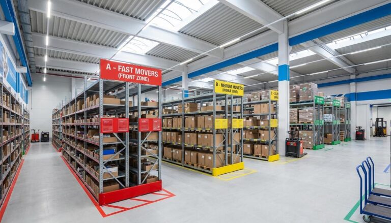
The action item here is simple. Do not try to solve this for every single item in your warehouse at once. Instead, start with your most valuable or high-volume products. We recommend using an ABC inventory classification to identify which items deserve this level of mathematical scrutiny. Once you have your “A” items, follow this step-by-step breakdown.

1. Gather your data: Pull your sales records from the last 12 months to determine annual demand. Ask your accounting team for a realistic estimate of what it costs to process one purchase order.
2. Calculate your holding rate: Determine your carrying cost percentage. Most experts suggest a rate between 20% and 30% of the item’s value. This covers everything from the cost of capital to warehouse utilities.
3. Run the calculation: Plug your numbers into the EOQ formula. Compare this result to your current ordering habits. Are you ordering far more or far less than the math suggests?
4. Adjust for lead time: The EOQ tells you how much to order. Use your lead time data to determine when to order. This ensures the new shipment arrives just as your current stock is hitting your safety limit.
5. Review periodically: Costs change. If your warehouse rent goes up or a supplier changes their shipping fees, your EOQ will change too. Recalculate at least once or twice a year.

Your next step is to look at your current inventory software. Many modern ERP systems have an EOQ field built-in. If you have been letting the system use a default setting, you might be surprised by how much you can save by entering your own verified data. Research from the NetSuite resource center suggests that even small adjustments to order sizes can significantly impact a company’s bottom line over a fiscal year.

Quick Reference: EOQ at a Glance

• Primary Goal: To find the order size that minimizes total inventory costs.
• Key Variables: Annual demand, ordering cost, and holding cost.
• The “Magic” Point: Where annual ordering costs and annual holding costs are equal.
• When to Use: Best for items with relatively stable demand and known costs.
• Main Benefit: Improved cash flow and reduced waste in the supply chain.
• Limitation: Does not inherently account for seasonality or shipping delays.

Common Questions About Economic Order Quantity

What happens if I order more than the EOQ?

The answer is that your total costs will increase because your holding costs will grow faster than your ordering cost savings. You will have more money tied up in stock, higher insurance premiums, and a greater risk of items expiring or becoming damaged in the warehouse.

Is EOQ still relevant with modern JIT systems?

Yes, and here is why. Even in Just-in-Time (JIT) environments, there is still a cost to “setup” or “order.” EOQ helps define how close to zero that setup cost needs to be to make ultra-small batches economical. It provides the mathematical target for your efficiency improvements.

How do I estimate the cost of an order?

The direct answer is to look at the total labor cost of your purchasing department and divide it by the number of orders they process annually. Add in any fixed shipping fees, inspection costs, and invoice processing fees to get a comprehensive “S” value for your formula.

Can EOQ be used for services?

Not quite. EOQ is specifically designed for physical goods that incur storage and handling costs. For services, you would look at different resource optimization models that focus on labor capacity and time management rather than physical lot sizes.

We have seen this question come up constantly, so let us settle it. The economic order quantity is one of the most reliable tools in a manager’s kit. It moves the conversation from “I think we need more” to “The data shows this is the most profitable path.” By balancing the desire to save on shipping with the reality of storage costs, you create a leaner, more resilient business. Use the formula, acknowledge the assumptions, and start optimizing your high-value SKUs today. The practical takeaway is that your inventory should be working for you, not just taking up space.